Modelling variance in reproductive success (VRS)

If we instead want some males to have higher reproductive success than others, this must modelled. This can be done in many ways, including a simple model that draws a reproductive success randomly to more advancde ones that models inheriting (possibly only parts of) your father’s reproductive success. Like any modelling choice this is important and should ideally reflect how the system you model works.

What we did in “How convincing is a matching Y-chromosome profile?” (2017) was the following as described in the subsection “Variable reproductive success” under “Materials and methods”: reproductive success is not inherited, but rather sampled randomly at each generation according to a Dirichlet distribution.

We modelled it with two parameters, \(\alpha\) and \(\beta\), that are parameters in a Gamma distribution with \(\alpha\) being the shape and \(\beta\) being the scale (not rate). (In our paper we use \(\beta = 1/\alpha\).) We then draw \(X_i \sim \text{Gamma}(\alpha, \beta)\) for \(i = 1, 2, \ldots, N\) as the relative probabilities with Var[\(X_i\)] = \(\alpha \beta^2\) (in our paper with \(\beta = 1/\alpha\) then Var[\(X_i\)] = \(1/\alpha\)). Sometimes \(\text{Gamma}(\alpha, 1)\) variables are sampled to sample a symmetric Dirichlet distribution, which then gives Var[\(X_i\)] = \(\alpha\).

set.seed(1) # For reproducibility

library(dirmult)

N <- 1000  # individuals
K <- 1000 # samples
alpha <- 5
beta <- 1/alpha

x <- replicate(K, rgamma(N, shape = alpha, scale = beta))
vrs <- apply(x, 1, var)
mean(vrs)    # simulated VRS

## [1] 0.20015

alpha*beta^2 # theoretical VRS

## [1] 0.2

y1 <- apply(x, 2, function(z) z / sum(z))
y2 <- t(dirmult::rdirichlet(K, alpha = rep(alpha, N)))

Now consider the distribution of the first element of the K simulations:

plot(density(y1[1, ]))
points(density(y2[1, ]), type = "l", col = "red")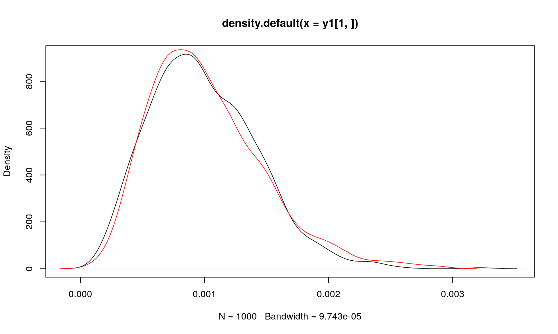

We expect that Var[\(Y_i\)] = \(\frac{(\alpha/(\alpha N))(1-(\alpha/(\alpha N))}{N\alpha + 1} = \frac{(1/N)(1-1/N)}{N\alpha + 1}\):

((1/N)*(1-1/N))/(N*alpha + 1)

## [1] 1.9976e-07

var(y1[1, ])

## [1] 1.857362e-07

var(y2[1, ])

## [1] 2.111156e-07

Standard deviation in offspring count (SDO)

How do we know what a given VRS values means in terms of the standard deviation in offspring count (SDO)? We can reason about that as follows. We can assume that in a population with fixed size, the number of children is approximately Poisson distributed (for large \(N\)) with parameter \(\lambda\) where the rate, \(\lambda\), is the reproductive success:

set.seed(1)
sdo <- replicate(1000, {
  lambda <- rgamma(N, shape = alpha, scale = beta)
  children <- rpois(N, lambda)
  mean(children) # Fixed size, mean should be 1
  sd(children)
})
mean(sdo)

## [1] 1.094051

Actually, we can go further: The Poisson rate \(\lambda\) is itself the Gamma(\(\alpha, \beta\)) distributed reproductive success.
So the offspring count is a Gamma-Poisson mixture or in other words follows a negative binomial distribution with parameters \(r = \alpha\) and \(p = \frac{\beta}{\beta + 1}\), such that the mean offspring count is \(pr/(1-p)\) and standard deviation in offspring count is \(\sqrt{pr/(1-p)^2}\):

r <- alpha
p <- beta/(beta + 1)
p*r/(1-p)

## [1] 1

sqrt(p*r/(1-p)^2)

## [1] 1.095445

So for \(\alpha = 5\) (and \(\beta = 1/\alpha = 0.2\)) VRS (variance in reproductive success) is 0.2 and SDO (standard deviation in offspring count) is about 1.1.

This relationship can be illustrated (for \(\beta = 1/\alpha\)):

alpha <- seq(0.1, 10, length.out = 100)
beta <- 1/alpha
# VRS
vrs <- 1/alpha
# SDO
r <- alpha
p <- beta/(beta + 1)
sdo <- sqrt(p*r/(1-p)^2)

plot(alpha, vrs, type = "l")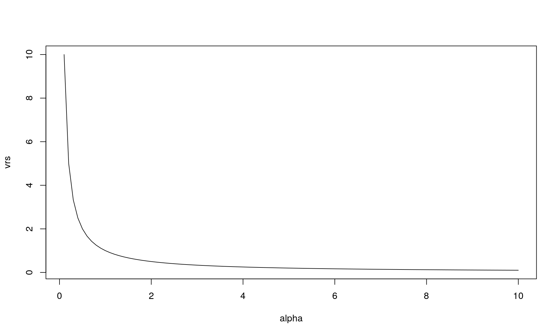

plot(alpha, sdo, type = "l")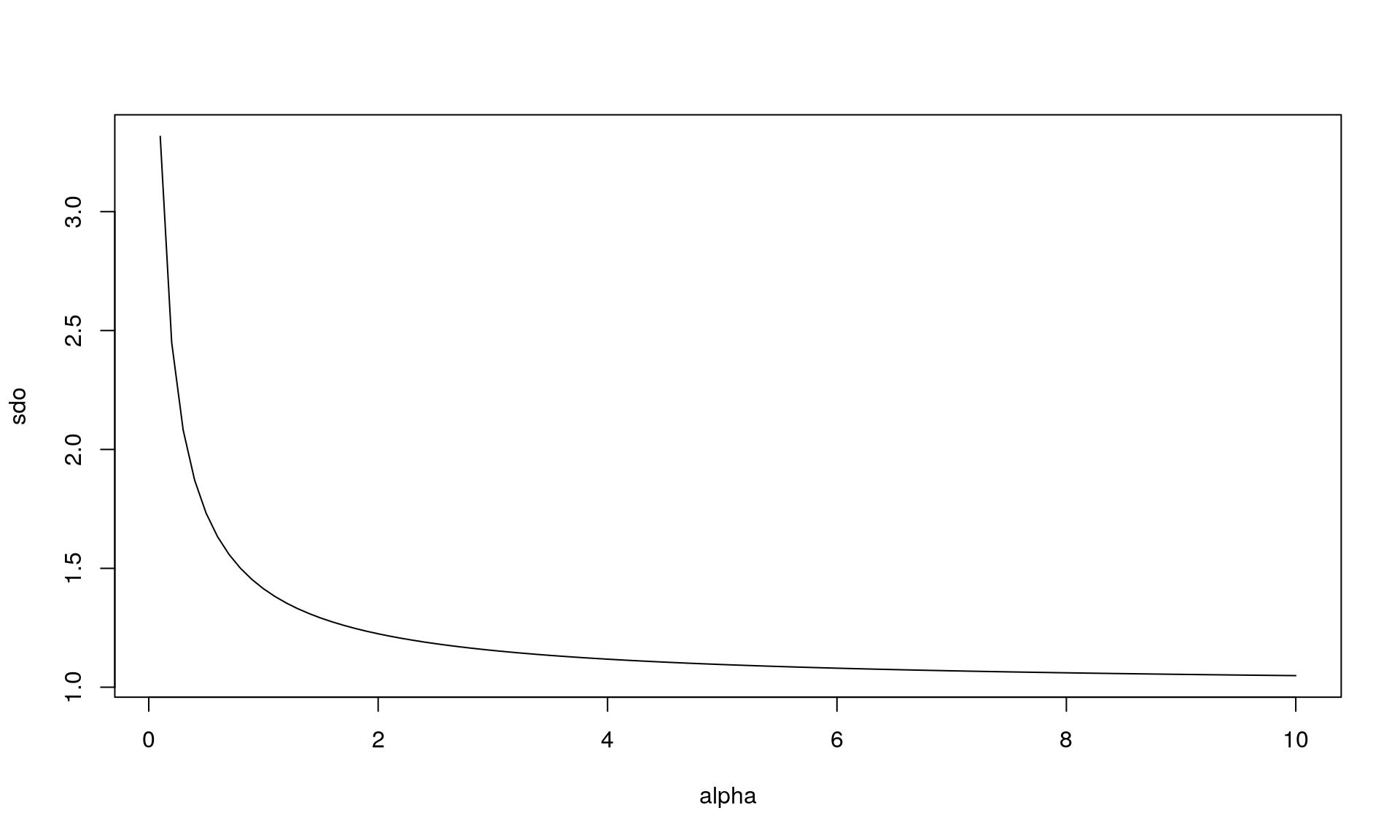

plot(vrs, sdo, type = "l")
abline(0, 1, lty = 2) # y = x is dashed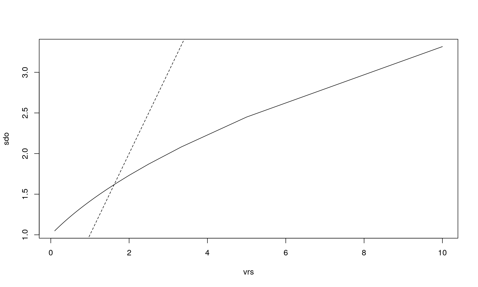

Simulating with standard deviation in offspring count

How do we then go the other way around: Say we have information about the offspring count in a population. How can we then simulate a population with this distribution? Well, in the model described above (assuming fixed population size), we can do something simple like this:

calc_sdo <- function(alpha) {
  beta <- 1/alpha
  r <- alpha
  p <- beta/(beta + 1)
  sdo <- sqrt(p*r/(1-p)^2)
  return(sdo)
}

find_alpha <- function(sdo) {
  f <- function(alpha) {
    calc_sdo(alpha) - sdo
  }
  
  alpha <- uniroot(f, interval = c(1e-10, 100))$root
  return(alpha)
}

calc_sdo(alpha = 5)

## [1] 1.095445

find_alpha(sdo = 1.095445)

## [1] 5.000013

For example:

offsping_counts <- rep(c(0, 0, 2, 0, 1, 3), 1000)
mean(offsping_counts) # Must be 1

## [1] 1

sdo_ex <- sd(offsping_counts)
sdo_ex

## [1] 1.154797

alpha_ex <- find_alpha(sdo = sdo_ex)
alpha_ex

## [1] 2.997993

set.seed(1)

library(malan)

sample_sdo <- function() {
  sim_res_fixed <- sample_geneology(population_size = 1e3, 
                                  generations = 2, 
                                  gamma_parameter_shape = alpha_ex,
                                  gamma_parameter_scale = 1 / alpha_ex,
                                  enable_gamma_variance_extension = TRUE,
                                  generations_full = 2,
                                  progress = FALSE)
  peds <- build_pedigrees(sim_res_fixed$population, progress = FALSE)
  
  all_generations <- sim_res_fixed$individuals_generations
  gen_number <- sapply(all_generations, malan::get_generation)
  
  indvs_prev_gen <- which(gen_number == 1L)
  fathers <- all_generations[indvs_prev_gen]
  
  child_count <- sapply(lapply(fathers, malan::get_children), length)
  #mean(child_count)
  sd(child_count)
}

sdo <- replicate(10, sample_sdo())
plot(density(sdo))
abline(v = sdo_ex)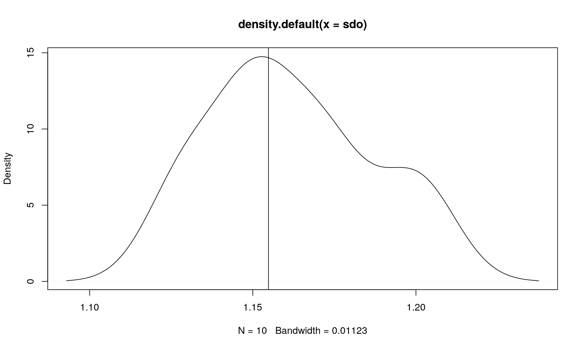

mean(sdo)

## [1] 1.16188

sdo_ex

## [1] 1.154797