Update Oct 14, 2019: Michael Höhle caught a mistake and notified me on Twitter. Thanks! The problem is that I used \(\text{Unif}(-10, 10)\) as importance distribution; this does not have infinite support as the target has. This is required, see e.g. Art B. Owen (2013), “Monte Carlo theory, methods and examples”. I have now updated the post to use a normal distribution instead.
Box plots are often used. They are not always the best visualisation (e.g. is bi-modality not visible), but I will not discuss that in this post.
Here, I will use it as an example of Importance sampling that is a technique to estimate tail probabilities without requiring many, many simulations.
Assume that we have a standard normal distribution. What is the probability of getting a box plot extreme outlier (here we use that it must be greater than 2.5 IQR from lower/upper quartile)?
This can be solved theoretically. And solving problems theoretically often yields great insight. But sometimes solving problems theoretically is impossible (or takes too long). So another way of solving problems is by using simulations. Here that way of solving the problem is demonstrated.
Solving directly
We can simulate it directly:
set.seed(2019)
x <- rnorm(10000)
qs <- quantile(x, c(0.25, 0.75))
# We know that it must be symmetric around 0, so take the average:
qs <- c(-1, 1)*mean(abs(qs))
iqr <- qs[2] - qs[1] # or IQR()
lwr <- qs[1] - 2.5*iqr
upr <- qs[2] + 2.5*iqr
indices <- x < lwr | x > upr
mean(indices)
## [1] 1e-04
So based on 10,000 simulations we believe the answer is around 1/10,000 = 0.01%. Because only one of the simulated values were outside the 2.5 IQR. Not too trustworthy…
Importance sampling
So we are trying to estimate a tail probability. What if we instead of simulating directly from the distribution of interest, we could simulate from some other distribution with more mass in the area of interest and then reweight the sample? That is the idea behind importance sampling.
So let us define the importance distribution as follows (it can be something else, too, e.g. a mixture of two normal distributions or something else):
imp_sd <- 10

rimp <- function(n) {
  rnorm(n, mean = 0, sd = imp_sd)
}

dimp <- function(x) {
  dnorm(x, mean = 0, sd = imp_sd)
}
Sampling is then done as follows:
set.seed(2019)
z <- rimp(2500)
We make a smaller sample to find limits (they are based on quartiles, which is fairly easy to estimate accurately by simulation):
qs <- quantile(rnorm(2500), c(0.25, 0.75))
# We know that it must be symmetric around 0, so take the average:
qs <- c(-1, 1)*mean(abs(qs))
iqr <- qs[2] - qs[1] # or IQR()
lwr <- qs[1] - 2.5*iqr
upr <- qs[2] + 2.5*iqr
Now, we do not count 0s (not outlier) and 1s (outlier) but instead consider importance weights, \(w(z) = f_X(z) / f_Y(z)\), where \(f_X(z)\) is the probability density function for a standard normal distribution and \(f_Y(z)\) is the probability density function for the importance distribution.
indices <- z < lwr | z > upr
mean(indices) # Now, a much larger fraction is in the area of interest
## [1] 0.6824
importance_weight <- dnorm(z) / dimp(z)
sum(importance_weight[indices]) / length(indices)
## [1] 4.88308e-05
So based on 2,500 + 2,500 simulations our estimate is now 0.0048831%.
It can (easily) be shown that the true answer is 0.005%.
Comparing approaches
We do both of the above 1,000 times to inspect the behaviour:
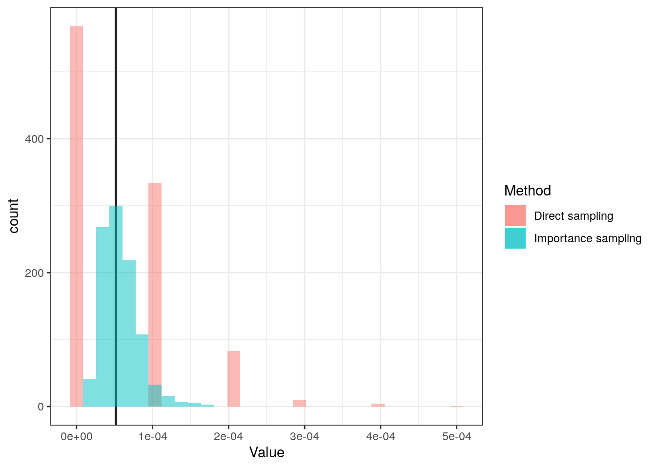
The reason that the density estimate for the direct method looks strange is because it only samples a few different values, and often does not get any outliers:
table(direct)
## direct
##     0 1e-04 2e-04 3e-04 4e-04 5e-04
##   568   334    83    10     4     1
The methods’ summaries are calculated:
| Method | Mean of estimates | SD of estimates | log10(MSE) |
|---|---|---|---|
| Direct sampling | 5.51e-05 | 7.36e-05 | -8.265658 |
| Importance sampling | 5.73e-05 | 2.43e-05 | -9.208113 |
As seen, on average both give the same answer (as expected), but the importance sampling provides a lower standard error.