Correlation is not transitive, in general at least

Update Aug 10, 2019: I wrote a new blog post about the same as below but using a simulation approach.

Update Aug 27, 2019: Minor change in how equations are solved (from version 0.9.0.9122).

Let \(\rho_{XY}\) be the correlation between the stochastic variables \(X\) and \(Y\) and similarly for \(\rho_{XZ}\) and \(\rho_{YZ}\). If we know two of these, can we say anything about the third?

Yes, sometimes, but not always. Say we have \(\rho_{XZ}\) and \(\rho_{YZ}\) and they are both positive. Intuition would then make us believe that \(\rho_{XY}\) is probably also positive then. But that is not always the case.

To see why, we need the partial correlation of \(X\) and \(Y\) given \(Z\): \[ \rho_{XY \mid Z}={\frac {\rho_{XY}-\rho _{XZ}\rho_{YZ}}{{\sqrt {1-\rho_{XZ}^{2}}}{\sqrt {1-\rho_{YZ}^{2}}}}} \]

The partial correlation between \(X\) and \(Y\) given \(Z\) means the correlation between \(X\) and \(Y\) with the effect of \(Z\) removed. Let us make a small example using the mtcars data:

x <- mtcars$mpg
y <- mtcars$drat
z <- mtcars$wt
cor(x, y)
## [1] 0.6811719
x_without_z <- residuals(lm(x ~ z))
y_without_z <- residuals(lm(y ~ z))
cor(x_without_z, y_without_z)
## [1] 0.1806278
(cor(x, y) - cor(x, z)*cor(y, z))/(sqrt(1 - cor(x, z)^2)*sqrt(1 - cor(y, z)^2))
## [1] 0.1806278

So the correlation between mpg (miles per gallon) and drat (rear axle ratio) is 0.6811719. And the partial correlation between mpg and draw given wt (weight in 1000 lbs) is 0.1806278.

We can rearrange the formula using Ryacas (see e.g. this blog post, note that it I’m using the development version that is currently only available via GitHub):

library(Ryacas)
pcor <- "rXYZ == (rXY - rXZ*rYZ)/(Sqrt(1 - rXZ^2)*Sqrt(1 - rYZ^2))"
rXY <- pcor %>% y_fn("Solve", "rXY") %>% yac_str()
rXY
## [1] "{rXY==(rXYZ-(-rXZ*rYZ)/(Sqrt(1-rXZ^2)*Sqrt(1-rYZ^2)))*Sqrt(1-rXZ^2)*Sqrt(1-rYZ^2)}"
rXY %>% y_rmvars() %>% yac_str()
## [1] "{(rXYZ-(-rXZ*rYZ)/(Sqrt(1-rXZ^2)*Sqrt(1-rYZ^2)))*Sqrt(1-rXZ^2)*Sqrt(1-rYZ^2)}"
rXY %>% y_fn("TeXForm") %>% yac_str()
## [1] "\\left( \\mathrm{ rXY } = \\left( \\mathrm{ rXYZ } - \\frac{ - \\mathrm{ rXZ } \\mathrm{ rYZ }}{\\sqrt{1 - \\mathrm{ rXZ } ^{2}} \\sqrt{1 - \\mathrm{ rYZ } ^{2}}} \\right)  \\sqrt{1 - \\mathrm{ rXZ } ^{2}} \\sqrt{1 - \\mathrm{ rYZ } ^{2}}\\right) "

\[\begin{align} \rho_{XY} &= \left( \rho_{XY \mid Z} - \frac{ - \rho_{XZ} \rho_{YZ}}{\sqrt{1 - \rho_{XZ}^{2}} \sqrt{1 - \rho_{YZ}^{2}}} \right) \sqrt{1 - \rho_{XZ}^{2}} \sqrt{1 - \rho_{YZ}^{2}} \\ &= \rho_{XY \mid Z} \sqrt{1 - \rho_{XZ}^{2}} \sqrt{1 - \rho_{YZ}^{2}} + \rho_{XZ} \rho_{YZ} \end{align}\]

The partial correlation takes values between \(-1\) and \(1\) so \(\rho_{XY}\) must lie in the interval \[ \rho_{XZ} \rho_{YZ} \pm \sqrt{1 - \rho_{XZ}^{2}} \sqrt{1 - \rho_{YZ}^{2}} . \]

Going back to the mtcars example:

rXZ <- cor(x, z)
rYZ <- cor(y, z)
rXZ*rYZ + c(-1, 1)*sqrt(1 - rXZ^2)*sqrt(1 - rYZ^2)
## [1] 0.2692831 0.9670285
cor(x, y)
## [1] 0.6811719

We can illustrate this

library(tidyverse)

grid <- expand.grid(
  rXZ = seq(-1, 1, len = 100),
  rYZ = seq(-1, 1, len = 100))

d <- grid %>% 
  as_tibble() %>% 
  mutate(
    rXY_l = rXZ*rYZ - sqrt(1 - rXZ^2)*sqrt(1 - rYZ^2),
  rXY_u = rXZ*rYZ + sqrt(1 - rXZ^2)*sqrt(1 - rYZ^2),
) %>% 
  mutate(rXY_sign = case_when(
    rXY_l < 0 & rXY_u < 0 ~ "-1",
    rXY_l > 0 & rXY_u > 0 ~ "1",
    TRUE ~ "?"
  ))

p <- ggplot(d, aes(rXZ, rYZ, fill = rXY_sign)) + 
  geom_tile() +
  scale_fill_manual(expression(paste("Sign of ", rho[XY])), 
                    values = c("-1" = "red", "1" = "blue", "?" = "grey")) +
  labs(x = expression(rho[XZ]),
       y = expression(rho[YZ])) +
  theme_bw() +
  coord_equal()
p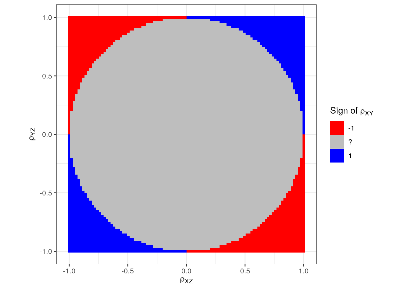

Interesting! We actually just found the circle with radius 1!

p + annotate("path",
   x = cos(seq(0, 2*pi, length.out = 100)),
   y = sin(seq(0, 2*pi, length.out = 100)),
   color = "green", size = 2)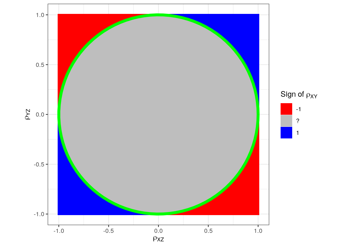

We can also argue mathematically: Before we found that \(\rho_{XY}\) must lie in the interval \[ \rho_{XZ} \rho_{YZ} \pm \sqrt{1 - \rho_{XZ}^{2}} \sqrt{1 - \rho_{YZ}^{2}} . \]

If \(\rho_{XY}\) must be positive, then we must have that both limits are greater than zero, namely that \[\begin{align} \rho_{XZ} \rho_{YZ} - \sqrt{1 - \rho_{XZ}^{2}} \sqrt{1 - \rho_{YZ}^{2}} &> 0 \\ \rho_{XZ} \rho_{YZ} + \sqrt{1 - \rho_{XZ}^{2}} \sqrt{1 - \rho_{YZ}^{2}} &> 0 . \end{align}\] We move the \(\sqrt{1 - \rho_{XZ}^{2}} \sqrt{1 - \rho_{YZ}^{2}}\) part on the other side of the equality sign and square both sides to obtain the same two equations, namely: \[\begin{align} \rho_{XZ}^2 \rho_{YZ}^2 &> \left ( 1 - \rho_{XZ}^{2}\right ) \left (1 - \rho_{YZ}^{2}\right ) \\ &= 1 - \rho_{XZ}^{2} - \rho_{YZ}^{2} + \rho_{XZ}^2 \rho_{YZ}^2 . \end{align}\] To summarise: If \(\rho_{XY}\) must be positive, then we must have that \[ \rho_{XZ}^{2} + \rho_{YZ}^{2} > 1 . \] Similar arguments can be used to show the same if \(\rho_{XY}\) must be negative.

In other words, if we have two known correlations, \(\rho_{XZ}\) and \(\rho_{YZ}\), then \[ \text{sign}(\rho_{XY}) = \begin{cases} \text{sign}(\rho_{XZ}) \text{sign}(\rho_{YZ}) & \rho_{XZ}^2 + \rho_{YZ}^2 > 1 \\ \text{not known} & \rho_{XZ}^2 + \rho_{YZ}^2 \leq 1. \end{cases} \] In other words, we only know the sign of the correlation when the two known correlations are sufficiently large (either positive or negative).

Again, going back to the mtcars example:

rXZ <- cor(x, z)
rYZ <- cor(y, z)
rXZ^2 + rYZ^2
## [1] 1.260404

So the sign of \(\rho_{XY}\) can be known and is positive because

sign(rXZ) * sign(rYZ)
## [1] 1

This was also known from calculating the limits earlier.

Terence Tao has a mathematical treatment of the topic in his blog post “When is correlation transitive?”.