Wolfe conditions for deciding step length in inexact line search: An example with the Rosenbrock function

Last updated on Sep 20, 2019 6 min read Statistics

In inexact line search (a numerical optimisation technique) the step length (or learning rate) must be decided. In connection to that the Wolfe conditions are central. Here I will give an example showing why they are useful. More on this topic can be read elsewhere, e.g. in the book of Nocedal and Wright (2006), “Numerical Optimization”, Springer.

Wolfe conditions

The Wolfe conditions consists of the sufficient decrease condition (SDC) and curvature condition (CC):

$\begin{aligned} (SDC) & f (x_{k} + α_{k} p_{k}) & \leq f (x_{k}) + c_{1} α_{k} \nabla f_{k}^{⊺} p_{k} \\ (CC) & \nabla f (x_{k} + α_{k} p_{k})^{⊺} p_{k} & \geq c_{2} \nabla f_{k}^{⊺} p_{k}, \end{aligned}$ with $0 < c_{1} < c_{2} < 1$ .

The strong Wolfe conditions are:

$\begin{aligned} (SDC) & f (x_{k} + α_{k} p_{k}) & \leq f (x_{k}) + c_{1} α_{k} \nabla f_{k}^{⊺} p_{k}, \\ (CC') & | \nabla f (x_{k} + α_{k} p_{k})^{⊺} p_{k} | & \leq c_{2} | \nabla f_{k}^{⊺} p_{k} |, \end{aligned}$ with $0 < c_{1} < c_{2} < 1$ .

Example

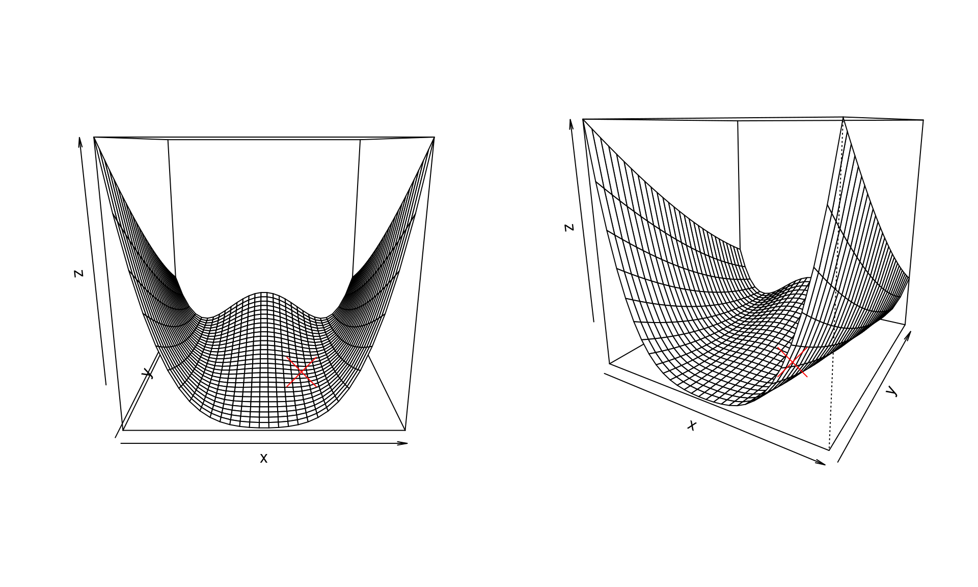
We use the Rosenbrock function to illustrate these conditions when choosing step length. We use a classic version, namely $f (x, y) = (1 - x)^{2} + 100 (y - x^{2})^{2}$ Its global minimum is at $(1, 1)$ and the gradient is $\nabla f (x, y) = (- 2 (1 - x) - 400 x (y - x^{2}), 200 (y - x^{2})) .$

A few illustrations of the function $f$ (the global minimum marked with a red cross):

Let $z = (x, y)$ and $z_{k} = (x_{k}, y_{k})$ , and further $f (z) = f (x, y)$ for easier notation. The line search is then $z_{k + 1} = z_{k} + α_{k} p_{k}$ for direction $p_{k}$ and step length $α_{k}$ . In determining the step length the function $Φ (α) = f (z_{k} + α p_{k})$ is often used. It tells us the value of the function we are minimising for any given step length $α$ . Recall that the current position is $z_{k}$ and the direction $p_{k}$ is chosen. The only thing left to choose is $α$ . So to make that more clear, we refer to $Φ (α)$ instead of $f (z_{k} + α p_{k})$ .

The aim is that $f (z_{k} + α p_{k}) < f (z_{k})$ , and if the direction chosen is a descent direction (e.g. the negative gradient), then for sufficiently small $α$ this will be possible. But just using $f (z_{k} + α p_{k}) < f (z_{k})$ as a criteria is not sufficient to ensure convergence, which is why the Wolfe conditions are used.

Now, say we start the line search at $z_{0} = (x_{0}, y_{0}) = (- 2.2, 3),$ then the gradient at that point is $\nabla f_{0} = \nabla f (z) |_{z = z_{0}} = (- 1625.6, - 368) .$

Say we to a line search from $z_{0} = (x_{0}, y_{0})$ in the direction of the negative gradient given by $p_{0} = (1625.6, 368) .$

In $z_{0} = (x_{0}, y_{0})$ we have that $Φ (α) = f (z_{0} + α p_{0}) .$

Note that for $α = 1$ then $z_{0} + α p_{0} = ((- 2.2) + (1625.6), (3) + (368)) = (1623.4, 371),$ so instead smaller values of $α$ are tried.

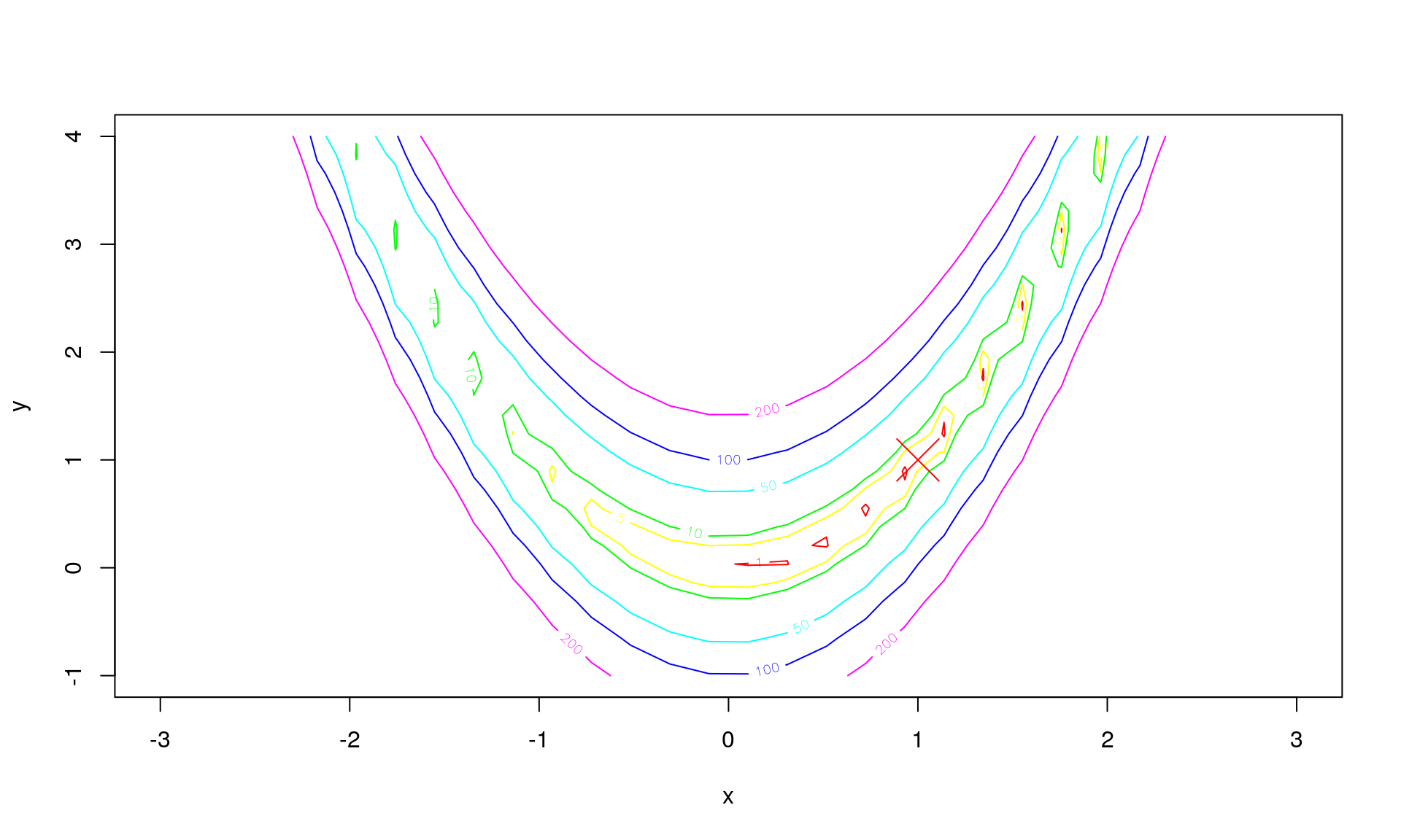
The path $z_{0} + α p_{0}$ for $α$ between $0$ and $0.003$ (chosen to make this example illustrative) is then:

This can instead be shown by visualising $Φ (α)$ instead as this is a univariate function, and $f$ can be difficult/impossible to visualise directly as in this example. For this example, $Φ (α)$ looks like this:

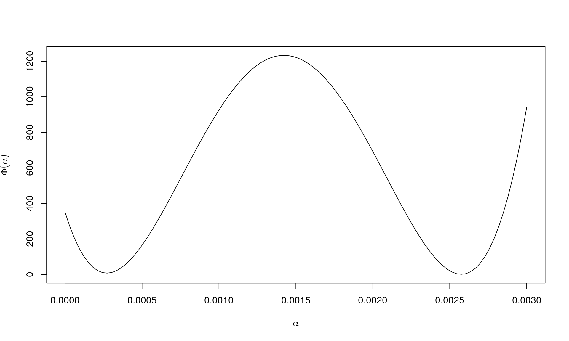
As seen, if $α$ is sufficiently small, then we move to a position with a smaller value for $f$ . But we can also end up in a place with a higher value (although we are moving in the descent direction).

The sufficient decrease condition

We now consider the Wolfe conditions. The SDC (sufficient decrease condition) is $\begin{matrix} (SDC) & Φ (α) = f (z_{k} + α p_{k}) \leq f (z_{k}) + c_{1} α \nabla f_{k}^{⊺} p_{k} \end{matrix}$ with $0 < c_{1} < 1$ . Let us disect this condition.

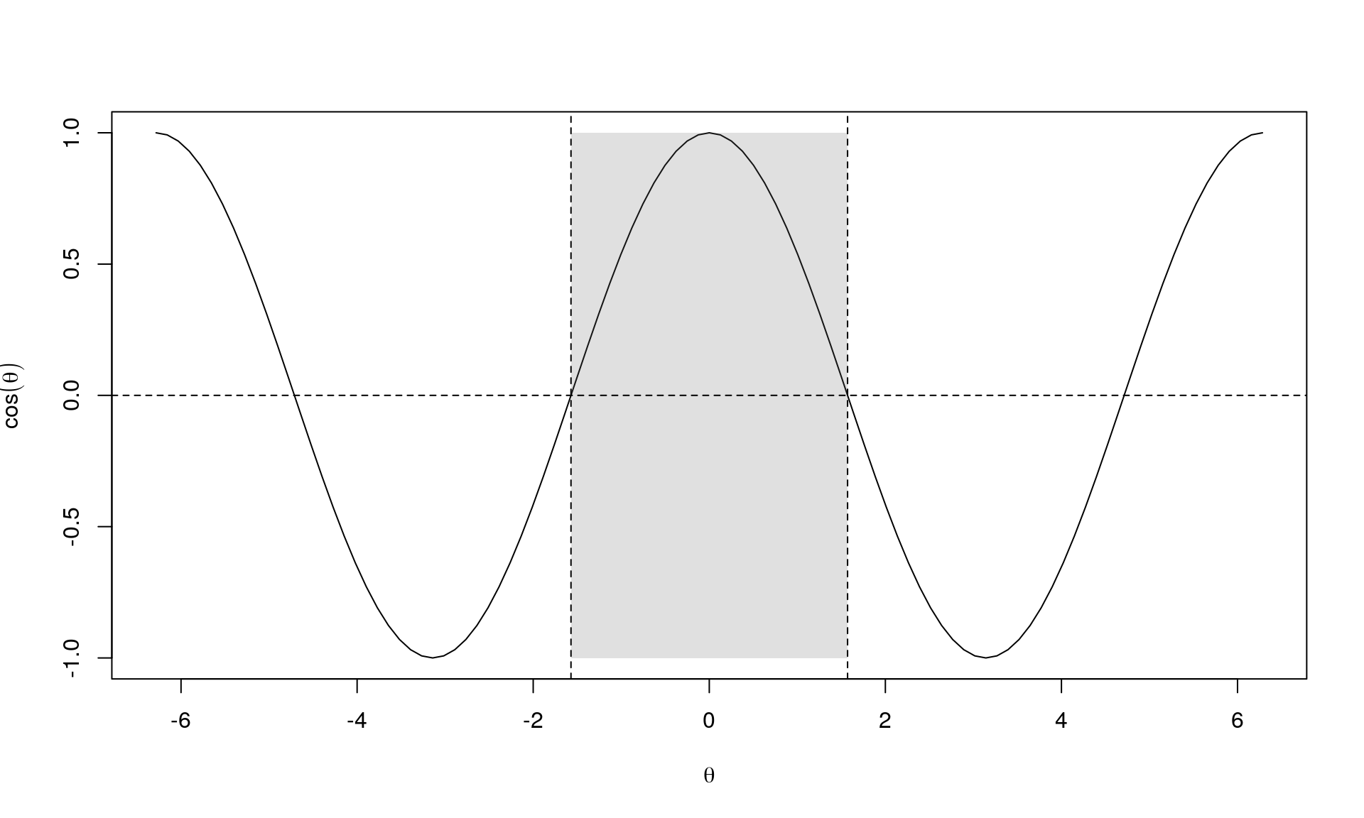
First, we focus on $\nabla f_{k}^{⊺} p_{k}$ . Note that $\nabla f_{k}^{⊺} p_{k} = p_{k} \cdot \nabla f_{k} = ‖ p_{k} ‖ ‖ \nabla f_{x} ‖ \cos (θ)$ (the latter equality in an Euclidian setting). What do we know about $θ$ ? We require that $p_{k}$ is a descent direction (“point in the same way as the negative gradient, $- \nabla f_{k}$ ”) and thus the angle between $p_{k}$ and the negative gradient, $- \nabla f_{k}$ , is $(- π / 2, π / 2)$ .

Instead of the negative gradient, we consider the gradient. So multiplying with $- 1$ means that $\nabla f_{k}^{⊺} p_{k} < 0$ .

Further, $f (z_{k})$ is a value in $R$ . And as $c_{1} > 0$ , $α > 0$ and $\nabla f_{k}^{⊺} p_{k} < 0$ we have that $c_{1} \nabla f_{k}^{⊺} p_{k} < 0$ . In other words, the condition can be written as $Φ (α) \leq β_{0} + α β_{1}$ where $β_{0} = f (z_{k})$ and $β_{1} = c_{1} \nabla f_{k}^{⊺} p_{k} < 0$ . So a stright line with negative slope.

In this case, $β_{0} = f (z_{0}) = 348.8$ and $β_{1} = c_{1} \nabla f_{k}^{⊺} p_{k}$ (using $p_{k} = - \nabla f_{k}$ ). See below for some choices of $c_{1}$ :

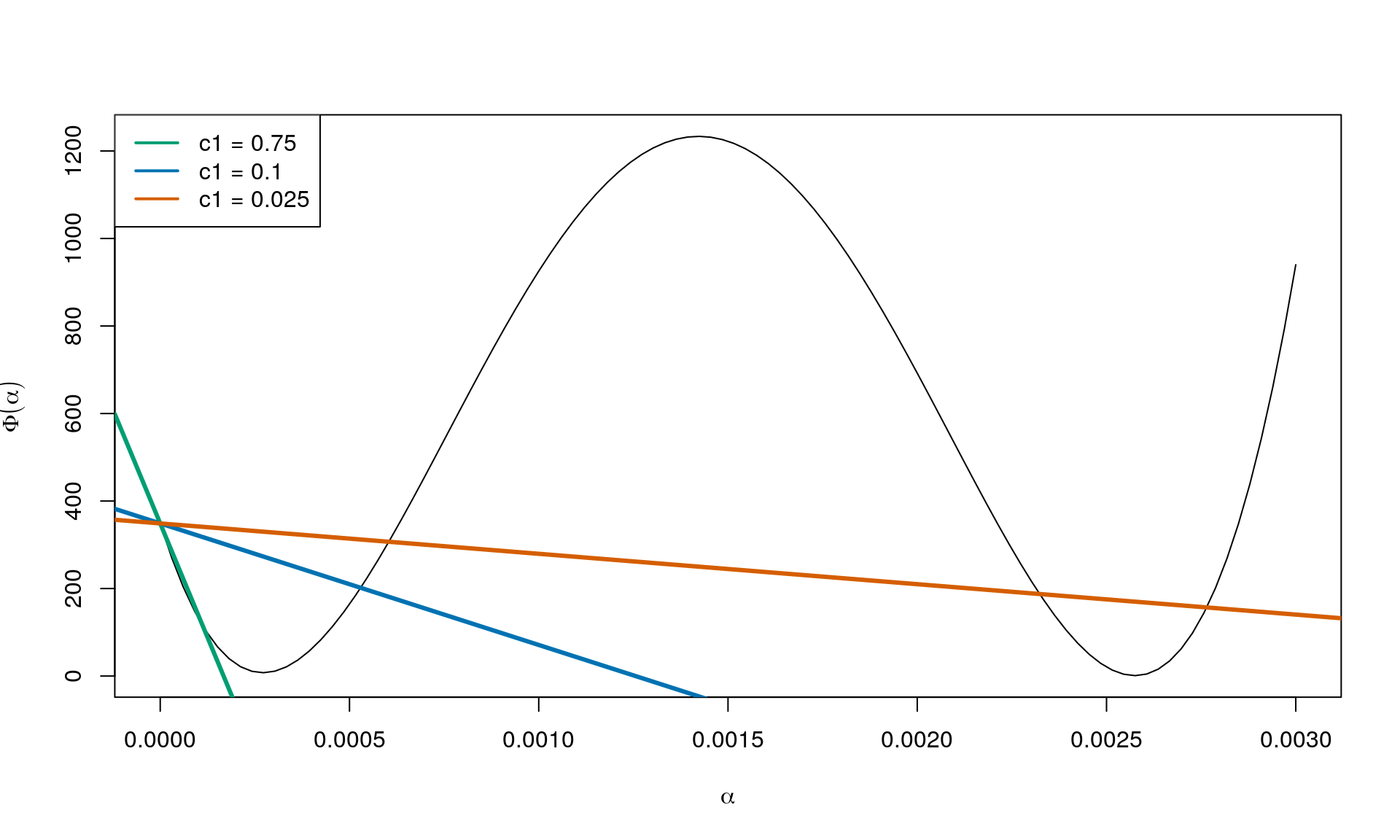
In other words, varying $c_{1}$ from $0$ to $1$ gives straight lines from $Φ (α) = f (z_{k})$ for $c_{1} = 0$ to $Φ (α) = f (z_{k}) + α \nabla f_{k}^{⊺} p_{k}$ for $c_{1} = 1$ , where the latter corresponds to the tangent of $Φ (α)$ at $α = 0$ .

To see this note that at $α = 0$ , the tangent to $Φ (α)$ is $c_{1} \nabla f_{k}^{⊺} p_{k}$ . This should be the same as the directional derivative of the objective function $f$ in the direction of $p_{k}$ . Which exactly happens for $c_{1} = 1$ .

So the factor $\nabla f_{k}^{⊺} p_{k}$ makes it possible to go from the extreme cases with a horizontal line to that of the directional derivative of the objective function $f$ in the direction of $p_{k}$ .

The curvature condition

The curvature condition (CC) is $\begin{matrix} (CC) & \nabla f (z_{k} + α_{k} p_{k})^{⊺} p_{k} \geq c_{2} \nabla f_{k}^{⊺} p_{k} . \end{matrix}$

We are in $z_{k}$ and looking in direction $p_{k}$ which is a descent direction. We know from before that $\nabla f_{k}^{⊺} p_{k} < 0$ , so it goes downhill from where we are now. We are looking for a critical point $z^{*}$ such that $\nabla f (z^{*}) = 0$ . So at the next point $z_{k + 1} = z_{k} + α_{k} p_{k}$ we think the gradient should be less negative than it is now; still looking in direction $p_{k}$ .

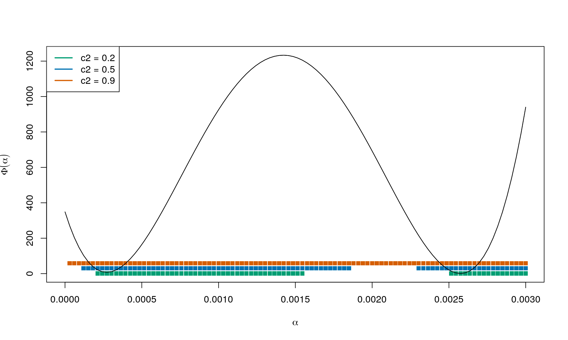
So the directional derivative at the next iterate continuing in the same direction as got us here has to be greater than $c_{2} \nabla f_{k}^{⊺} p_{k}$ , with $c_{2}$ controlling the expression to range from 0 to $\nabla f_{k}^{⊺} p_{k}$ , i.e. the directional derivative where we are standing now ( $z_{k}$ ).

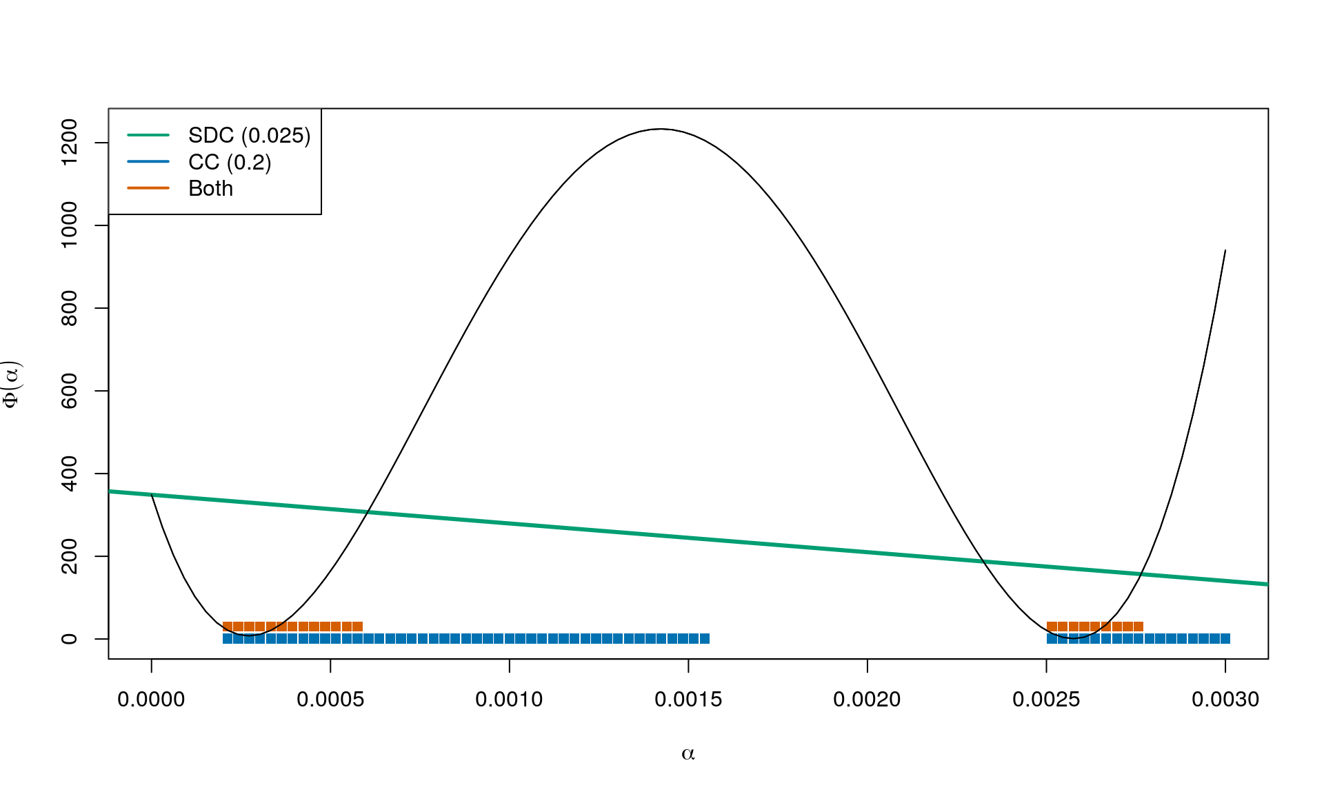
Combining

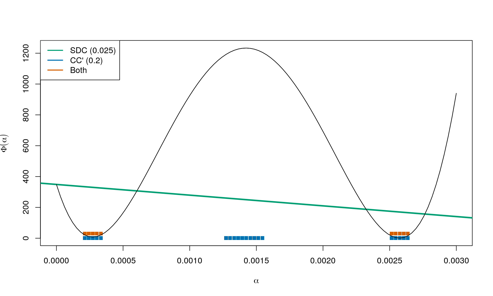
Result for $c_{1} = 0.025$ and $c_{2} = 0.2$ :

The strong Wolfe conditions

The curvature condition in the strong Wolfe conditions is:

$\begin{matrix} (CC') & | \nabla f (z_{k} + α_{k} p_{k})^{⊺} p_{k} | \leq c_{2} | \nabla f_{k}^{⊺} p_{k} | . \end{matrix}$

This is very similar to CC, except now the directional derivative at the next iterate continuing in the same direction as got us here cannot be too positive.

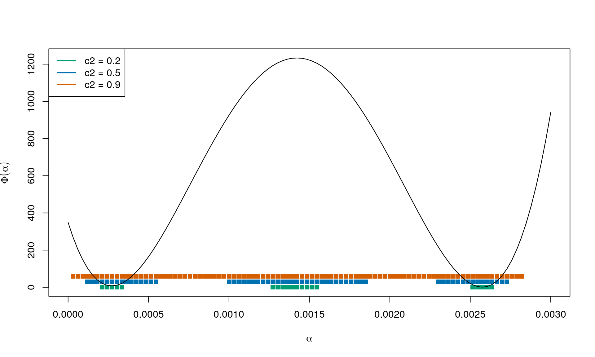
Again combining with $c_{1} = 0.025$ and $c_{2} = 0.2$ we obtain:

Summary

Small values of $c_{1}$ (close to 0) means that we can go far (limited almost only by a horizontal line). Large values of $c_{2}$ (close to 1) means that the directional derivative in the next iterate can be almost as negative as it currently is.

R Statistics

Mikkel Meyer Andersen

Assoc. Professor of Applied Statistics

My research interests include applied statistics and computational statistics.