Problem that must be solved

We imagine someone is hungry for both pizza and frozen yogurt. The conditions are as follows:

• A budget of $45 and must spend it all.
• A slice of Hawaiian pizza costs $3.
• A bowl of frozen yogurt costs $1.50.

The number of pizza slices that will be bought is denoted by \(x\) and the number of bowls of frozen yogurt that will be bought is denoted by \(y\).

The happiness from eating pizza and frozen yogurt is assumed to follow this utility function: \[ U(x, y) = x^2 \cdot \frac{1}{4} y \]

The budget line

First we load a few packages:

library(tidyverse)
library(wesanderson) # for wes_palette
library(Ryacas)

theme_set(theme_bw()) # I like this theme

Recall that we need to find \((x, y)\) such that \(3x + 1.5y = 45\) (using the entire budget) where \(U(x, y)\) is maximal (most happy).

The line \(3x + 1.5y = 45\) is called the budget line: it separates the solutions spending less than the budget and more than the budget. (There are some technicalities in not being able to buy fractional amounts of pizza/yogurt, but that is not central and the numbers are chosen to avoid this.)

To find the straight line, we see what happens if all the money is spent on either pizza or frozen yogurt:

total_budget <- 45
price_x <- 3
price_y <- 1.5
n_pizza <- total_budget / price_x
n_pizza
## [1] 15
n_yogurt <- total_budget / price_y
n_yogurt
## [1] 30

So the person can either buy 15 pizza slices or 30 frozen yogurts.

The \(x\) axis denotes the number of pizza slices, and the \(y\) axis denotes the number of bowls of frozen yogurt. The intercept of the budget line is where \(x=0\), i.e. if not buying pizza slices and only buying bowls of frozen yogurt. So the intercept of the budget line is 30. The slope is how much \(y\) changes when \(x\) changes by \(1\). We have calculated the two points \(p_1 = (x_1, y_1) = (0, 30)\) and \(p_2 = (x_2, y_2) = (15, 0)\). So the slope is: \[ \frac{y_2 - y_1}{x_2 - x_1} = \frac{0 - 30}{15 - 0} = \frac{-30}{15} = -2 . \] Or in R:

slope <- -n_yogurt / n_pizza
slope
## [1] -2

Thus, the equation for the budget line is \[ y = -2x + 30 \] and can be drawn as follows:

budget <- function(x) (slope * x) + n_yogurt

under_region <- tribble(
  ~ x, ~ y,
  0, 0,
  0, n_yogurt,
  n_pizza, 0
) %>% mutate(Region = "Under-spending")
over_region <- tribble(
  ~ x, ~ y,
  0, n_yogurt,
  0, 100*n_yogurt,
  100*n_pizza, 100*n_yogurt,
  100*n_pizza, 0,
  n_pizza, 0
) %>% mutate(Region = "Over-spending")

regions <- bind_rows(under_region,
                     over_region)
regions_colors <- c("Under-spending" = "green", 
                    "Over-spending" = "red")

p <- ggplot() + 
  geom_polygon(data = regions, aes(x = x, y = y, fill = Region), alpha = 0.25) +
  # Draw the line
  stat_function(data = tibble(x = 0:15), aes(x = x),
                fun = budget, size = 1.5) +
  # Add a label
  annotate(geom = "label", x = 2.5, y = budget(2.5), 
           label = "Budget") +
  labs(x = "Slices of pizza", y = "Bowls of frozen yogurt") +
  # Make the axes go all the way to zero
  scale_x_continuous(expand = c(0, 0), breaks = seq(0, 15, 5)) +
  scale_y_continuous(expand = c(0, 0), breaks = seq(0, 30, 10)) +
  coord_cartesian(xlim = c(0, 16), ylim = c(0, 32))  +
  scale_fill_manual(values = regions_colors)
p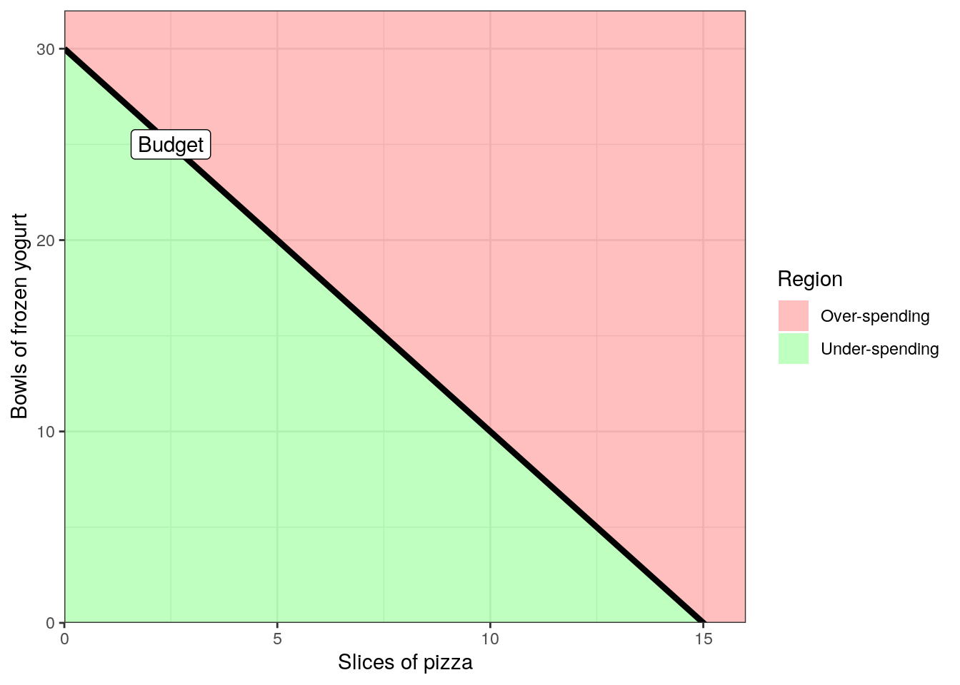

The utility function

Recall that utility (happiness from eating pizza and frozen yogurt) was given by \[ U(x, y) = x^2 \cdot \frac{1}{4} y . \]

This is also defined as an R function:

utility_u <- function(x, y) x^2 * (y / 4)

# 3 pizza slices, 8 yogurt bowls
utility_u(3, 8)
## [1] 18

The utility function defines a surface. We can choose to draw the directly or plot lines of \((x, y)\) values that give the same utility. First I will draw a few lines and then afterwards draw the surface.

To draw a line of \((x, y)\) values that give the same utility, we need to keep \(U\) fixed at some value. And then given \(U\) and \(x\), we can find \(y\). Here Ryacas comes in handy:

U <- "x^2 * (y/4)"
#Or automatically from the function:
#U <- as.character(as.expression(body(utility_u)))
U
## [1] "x^2 * (y/4)"
cmd <- U %>% paste0(" == U") %>% y_fn("Solve", "y")
cmd
## [1] "Solve(x^2 * (y/4) == U, y)"
utility_y_body <- yac_str(cmd) %>% y_rmvars() %>% y_fn("Simplify") %>% yac_str()
utility_y_body
## [1] "{(4*U)/x^2}"
utility_y_body_expr <- utility_y_body %>% yac_expr()
utility_y <- function(x, U) {
  eval(utility_y_body_expr, list(U = U, x = x))
}

Now, we can draw a few lines:

draw_U_line <- function(p, Uval) {
  Uname <- paste0("U = ", Uval)
  
  Udata <- tibble(x = seq(1, 16, len = 100), 
                  y = utility_y(x, U = Uval),
                  U = Uname)
  
  # Get position near y = 15
  label_data <- Udata %>% top_n(1, -abs(y - 15))
  
  p <- p + 
    geom_line(data = Udata, 
              aes(x = x, y = y, color = U), 
              size = 2) +
    geom_label(data = label_data, aes(x = x, y = y, 
                                      label = U, color = U), 
               show.legend = FALSE)
  
  return(p)
}

p2 <- p
for (Uval in c(10, 100, 500)) {
  p2 <- draw_U_line(p2, Uval)
}
p2 <- p2 + scale_color_brewer(palette = "Dark2")
p2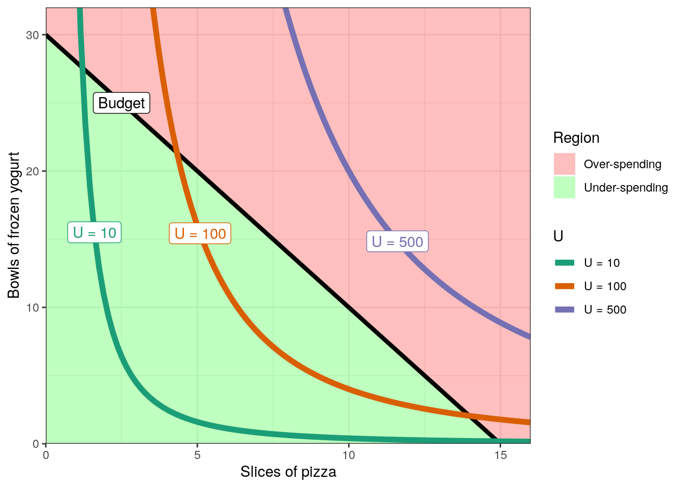

As mentioned, another option is to draw the surface (around the budget – remember the budget must be used exactly):

grid <- expand.grid(x = seq(0, 16, length.out = 100),
                    y = seq(0, 32, length.out = 100))
grid$budget <- with(grid, 3*x + 1.5*y)
grid <- subset(grid, abs(budget - 45) <= 10) # For more informative colouring
grid$U <- unlist(lapply(seq_len(nrow(grid)), function(i) {
  utility_u(grid$x[i], grid$y[i])
}))

p3 <- ggplot() + 
  geom_tile(data = grid, aes(x = x, y = y, fill = U)) +
  # Draw the line
  stat_function(data = tibble(x = 0:15), aes(x = x),
                fun = budget, size = 1.5) +
  # Add a label
  annotate(geom = "label", x = 2.5, y = budget(2.5), 
           label = "Budget") +
  labs(x = "Slices of pizza", y = "Bowls of frozen yogurt") +
  # Make the axes go all the way to zero
  scale_x_continuous(expand = c(0, 0), breaks = seq(0, 15, 5)) +
  scale_y_continuous(expand = c(0, 0), breaks = seq(0, 30, 10)) +
  coord_cartesian(xlim = c(0, 16), ylim = c(0, 32))  +
  scale_fill_gradientn(colours = wes_palette("Zissou1", 100, type = "continuous")) 
p3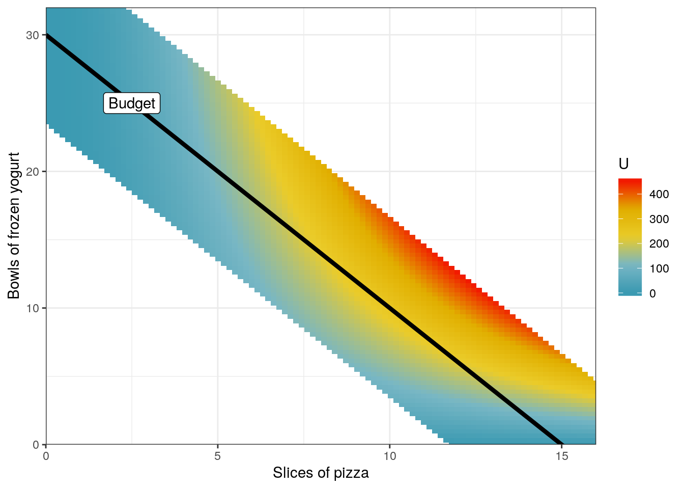

This indicate, based on the colors, that we expect that the maximal utility that can be attained is around 200-300.

Finding the optimal consumption

We need as high utility as possible constrained with hitting the budget exactly.

The original blog post has several economic explanations of what must be done. Please read it. Here I take the mathematical approach (and avoid explaning it in economic terms).

Thus we need to find max of \(U(x, y)\) along the budget line.

This is a typical example of Lagrange multipliers that can be used to find critical points in such situations. In this langugage, the optimisation problem that must be solved is to maximise \(U(x, y)\) subject to \(g(x, y) = 3x + 1.5y = k = 45\).

By using Lagrange multipliers, the optimisation problem can be converted to an unconstrained optimisation problem, namely finding the maximum of \[\begin{align} \mathcal{L}(x, y, a) &= U(x, y) - a(3x + 1.5y - 45) \\ &= x^2 (y/4) - a(3x + \frac{3}{2} y - 45) \end{align}\] where \(\frac{3}{2}\) is used instead of the floating-point representation 0.5 and \(a\) used instead of the traditional \(\lambda\).

We define this in R:

L <- "x^2 * (y/4) - a*(3*x + 3*y/2 - 45)"

Such an unconstrained optimisation problem is solved by finding critical points (and checking in what way they are critical). Critical points are found by solving the system of equations where the partial derivatives are equal to zero. Unfortunately, yacas’s Solve() and OldSolve() cannot solve this as seen here (included because the solver may work on other problems or may be improved):

Update Aug 27, 2019: I wrote a new blog post showing that Ryacas can now solve the system of equations directly without using optim().

# Either finding the partial derivates separately
eq1 <- paste0("D(x) ", L) %>% yac_str() %>% paste0(" == 0")
eq1
## [1] "(x*y)/2-3*a == 0"
eq2 <- paste0("D(y) ", L) %>% yac_str()  %>% paste0(" == 0")
eq2
## [1] "x^2/4-(3*a)/2 == 0"
eq3 <- paste0("D(a) ", L) %>% yac_str() %>% paste0(" == 0")
eq3
## [1] "45-(3*x+(3*y)/2) == 0"
eqsvec <- c(eq1, eq2, eq3)
eqs <- paste0("{", paste0(eqsvec, collapse = ", "), "}")
eqs
## [1] "{(x*y)/2-3*a == 0, x^2/4-(3*a)/2 == 0, 45-(3*x+(3*y)/2) == 0}"
# ...or directly using JacobianMatrix()
eqs <- paste0("{", L, "}") %>% # necessary to supply function as list
  y_fn("JacobianMatrix", "{x, y, a}") %>% 
  yac_str() %>% 
  y_fn("Nth", "1") %>% 
  yac_str() %>% 
  as_r() %>% 
  paste0(" == 0") %>% 
  as_y()
eqs
## [1] "{(x*y)/2-3*a == 0, x^2/4-(3*a)/2 == 0, 45-(3*x+(3*y)/2) == 0}"
cmd <- eqs %>% y_fn("OldSolve", "{x, y, a}") 
cmd
## [1] "OldSolve({(x*y)/2-3*a == 0, x^2/4-(3*a)/2 == 0, 45-(3*x+(3*y)/2) == 0}, {x, y, a})"
cmd %>% yac_str()
## [1] "{{x==(6*a)/y,y==(6*a)/Sqrt(6*a),a==a}}"

Instead, we do it numerically by taking the objective function, \(f\) say, to be the sum of the squared partial derivatives. When \(f(x, y, a)\) hits zero, it means that the all partial derivatives are zero. And it cannot be less than zero. So the objective function has a minimum where \(\mathcal{L}(x, y, a)\) has a critical point.

obj_fun <- c(paste0("D(x) ", L),
             paste0("D(y) ", L),
             paste0("D(a) ", L))
obj_fun
## [1] "D(x) x^2 * (y/4) - a*(3*x + 3*y/2 - 45)"
## [2] "D(y) x^2 * (y/4) - a*(3*x + 3*y/2 - 45)"
## [3] "D(a) x^2 * (y/4) - a*(3*x + 3*y/2 - 45)"
obj_fun <- paste0("(", obj_fun, ")^2", collapse = "+") %>% 
  y_fn("Simplify") %>% 
  yac_str()
obj_fun
## [1] "(x^4+4*x^2*y^2+(-12)*x^2*a+144*x^2+(-48)*x*y*a+144*x*y-4320*x+36*y^2-2160*y+180*a^2+32400)/16"

Or in a (maybe?) more readable format using y_fn("TeXForm"): \[ f(x, y, a) = \frac{x ^{4} + 4 x ^{2} y ^{2} - 12 x ^{2} a + 144 x ^{2} - 48 x y a + 144 x y - 4320 x + 36 y ^{2} - 2160 y + 180 a ^{2} + 32400}{16} \]

And enable it for computations in R by getting an R expression:

obj_fun_expr <- obj_fun %>% yac_expr()
obj_fun_expr
## expression((x^4 + 4 * x^2 * y^2 - 12 * x^2 * a + 144 * x^2 - 
##     48 * x * y * a + 144 * x * y - 4320 * x + 36 * y^2 - 2160 * 
##     y + 180 * a^2 + 32400)/16)

We can either to it without using the gradient of the objective function:

obj_fun_num <- function(par) {
  x <- par[1]
  y <- par[2]
  a <- par[3]
  
  val <- eval(obj_fun_expr, list(x = x, y = y, a = a))
  return(val)
}
opt_res1 <- optim(par = c(1, 1, 1), 
                  fn = obj_fun_num, 
                  method = "Nelder-Mead")
opt_res1
## $par
## [1]  9.999853 10.000484 16.667265
## 
## $value
## [1] 2.760206e-06
## 
## $counts
## function gradient 
##      216       NA 
## 
## $convergence
## [1] 0
## 
## $message
## NULL

Or by using the gradient:

obj_fun_grad <- paste0("{", obj_fun, "}") %>% # necessary to supply function as list
  y_fn("JacobianMatrix", "{x, y, a}") %>% 
  y_fn("Simplify") %>% 
  yac_expr()
obj_fun_grad
## expression(rbind(c((x^3 + 2 * x * y^2 + -6 * x * a + 72 * x + 
##     -12 * y * a + 36 * y - 1080)/4, (x^2 * y + -6 * x * a + 18 * 
##     x + 9 * y - 270)/2, (3 * (30 * a + -4 * x * y - x^2))/4)))
obj_fun_grad_num <- function(par) {
  x <- par[1]
  y <- par[2]
  a <- par[3]
  
  val <- c(eval(obj_fun_grad, list(x = x, y = y, a = a)))
  return(val)
}
opt_res2 <- optim(par = c(1, 1, 1), 
                  fn = obj_fun_num, 
                  gr = obj_fun_grad_num, 
                  method = "BFGS")
opt_res2
## $par
## [1] 10.00000 10.00000 16.66667
## 
## $value
## [1] -1.364242e-12
## 
## $counts
## function gradient 
##       72       18 
## 
## $convergence
## [1] 0
## 
## $message
## NULL

Both end up with \[ (x, y, a) = (10, 10, 16.6667) \] as a critical point. Or rather as \(16.6667\) is the floating-point representation something that is possibly \(16+2/3\) and that is

yac_str("16+2/3")
## [1] "50/3"

So probably the critical point is \[ (x, y, a) = (10, 10, 50/3) . \]

We now verify that the objective function is indeed 0 here (using yacas’s WithValue()), which is by construction the minimum:

cmd <- paste0("WithValue({x, y, a}, {10, 10, 50/3}, ", obj_fun, ")")
cmd
## [1] "WithValue({x, y, a}, {10, 10, 50/3}, (x^4+4*x^2*y^2+(-12)*x^2*a+144*x^2+(-48)*x*y*a+144*x*y-4320*x+36*y^2-2160*y+180*a^2+32400)/16)"
cmd %>% yac_str()
## [1] "0"

We also verify that it indeed is a minimum (by finding the Hessian and evaluating it in the critical point):

cmd <- paste0("HessianMatrix(", obj_fun, ", {x, y, a})")
cmd
## [1] "HessianMatrix((x^4+4*x^2*y^2+(-12)*x^2*a+144*x^2+(-48)*x*y*a+144*x*y-4320*x+36*y^2-2160*y+180*a^2+32400)/16, {x, y, a})"
H <- cmd %>% yac_str()
H %>% as_r()
##      [,1]                         [,2]                   
## [1,] "(12*x^2+8*y^2-24*a+288)/16" "(8*x*2*y-48*a+144)/16"
## [2,] "(8*x*2*y-48*a+144)/16"      "(8*x^2+72)/16"        
## [3,] "(-(24*x+48*y))/16"          "(-48*x)/16"           
##      [,3]               
## [1,] "(-(24*x+48*y))/16"
## [2,] "(-48*x)/16"       
## [3,] "45/2"

Or in a more readable format using y_fn("TeXForm"): \[ H = \left( \begin{array}{ccc} \frac{12 x ^{2} + 8 y ^{2} - 24 a + 288}{16} & \frac{16 x y - 48 a + 144}{16} & \frac{ - \left( 24 x + 48 y\right) }{16} \\ \frac{16 x y - 48 a + 144}{16} & \frac{8 x ^{2} + 72}{16} & \frac{ - 48 x}{16} \\ \frac{ - \left( 24 x + 48 y\right) }{16} & \frac{ - 48 x}{16} & \frac{45}{2} \end{array} \right) \]

We now inspect the eigenvalues at the critical point:

Hcrit <- paste0("WithValue({x, y, a}, {10, 10, 50/3}, ", H, ")") %>% 
  yac_expr() %>% eval()
Hcrit
##      [,1]  [,2]  [,3]
## [1,]  118  59.0 -45.0
## [2,]   59  54.5 -30.0
## [3,]  -45 -30.0  22.5
eigen(Hcrit, only.values = TRUE)
## $values
## [1] 172.684902  19.626396   2.688702
## 
## $vectors
## NULL

As all the eigenvalues are all positive, then the critical point is a local minimum.

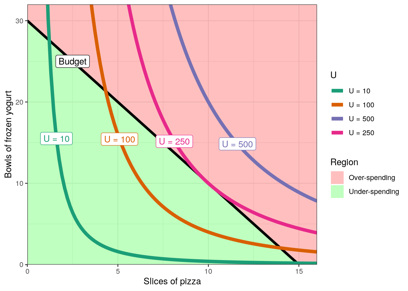
Now we can state that with the given budget, the optimal quantities are \(x=10\) pizza slices and \(y=10\) yogurt bowls yielding a utility of

utility_u(10, 10)
## [1] 250

And we include that line in the figure:

p4 <- p
for (Uval in c(10, 100, 250, 500)) {
  p4 <- draw_U_line(p4, Uval)
}
p4 <- p4 + scale_color_brewer(palette = "Dark2", 
                              limits = c("U = 10", "U = 100", "U = 500", "U = 250"))
p4